Theta Trend

Some background:

Let’s face it, technology has made it possible to access a wide range of tools for developing, backtesting, and optimizing systems. However, a simple (but powerful) tool like excel is a great way to validate a trading system. In this example we’re going to be keeping things really simple and backtesting a monthly ETF rotation system using 5 symbols that significantly outperforms buy and hold. All you need is Excel and an Internet connection. If you’re reading this, I’m guessing you have the Internet connection.  This post assumes you have a basic understanding of Excel, but you don’t need to be an expert.  You can either build the Excel file yourself by following the steps below or download it here.

Feel free to distribute the file, but please provide a link back to this post if you do.

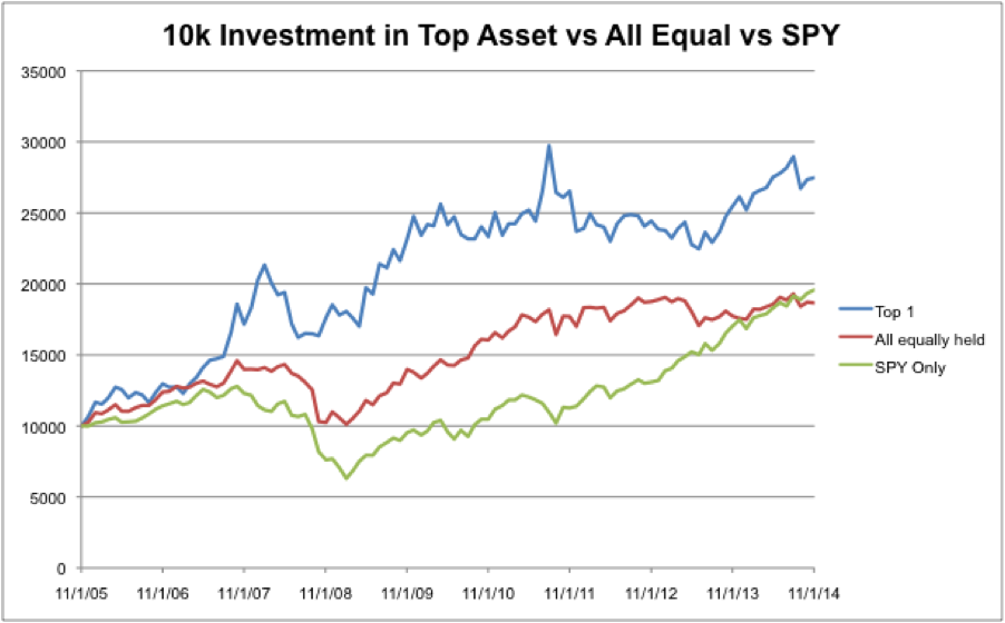
ETF Rotation System Excel

Once you’re done with the steps below, you’ll be able to chart your results and get a picture of how the system really performs.  The chart below is an example of a 5 ETF rotation system that ranks and buys the top ETF every month.  That performance is compared to buying and holding all ETF’s equally (without rebalancing) and holding the S&P 500 ($SPY).  You’ll find the exact calculation in Excel, but for the 9 year period tested the ETF Rotation system generated an annual return of 11.88% vs 7.75% for SPY and 7.18% for all held equally.

It’s worth noting that the way the excel file is constructed does not lend itself well to scaling up.  However, if you have some Visual Basic skills and a little creativity, you should be able to come up with a way to scale it.

Step 1: Choose Markets

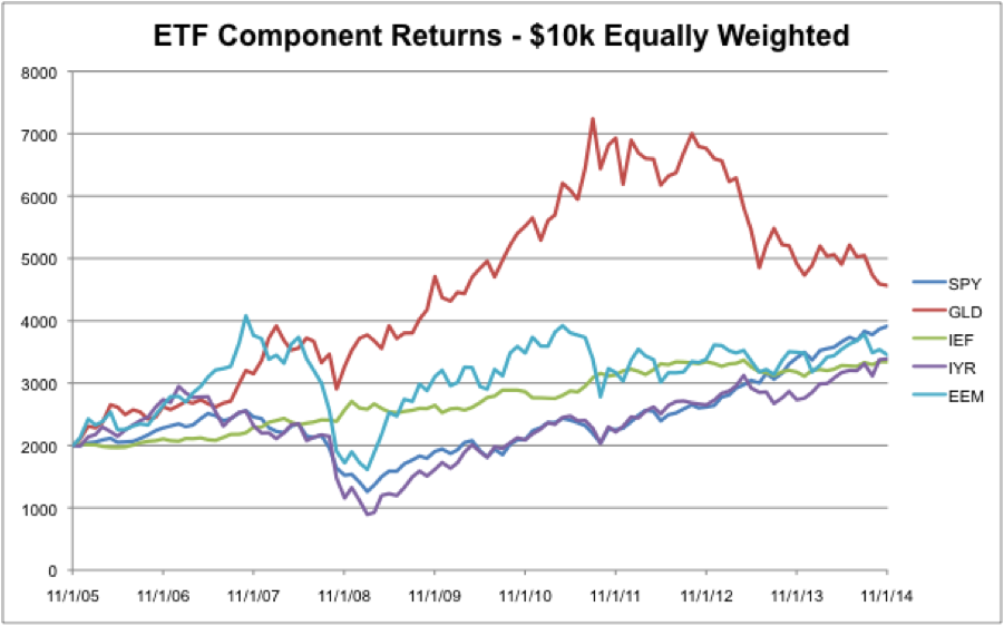
Choosing markets is a critical decision for all systems. Since I have a strong preference for trend following trading, we’re going to use a diversified group of markets. That being said, you could also consider using stock market sectors (Technology, Healthcare, etc), various commodities, or something completely different. I wanted to use relatively uncorrelated markets with around 10 years of historical data so I’m going to be using the following ETF’s:

• SPY – S&P 500
• GLD – Gold
• IEF – 10 Year Treasury
• IYR – US Real Estate
• EEM – Emerging Markets

The image below shows the individual ETF returns over the test period:

Step 2: Collect and Consolidate Data

Once you’ve decided on the markets, you’ll need to fire up Excel and find a source for historical data. In the interest of frugality, let’s use free data from Yahoo Finance.  Just a reminder that the construction of this particular spreadsheet doesn’t scale extremely well so fewer symbols will be easier to execute. That being said, with some creativity and skills in Visual Basic you could make the test more dynamic.

When you head over to Yahoo Finance, you can enter one of the symbols you’ve chosen and get a quote. On the quote page, click the link on the left for “Historical Data.” On the Historical Data page, select monthly data and submit. If you scroll to the bottom of the monthly data there is a link to download the data to a spreadsheet. Download monthly historical data for all of the symbols in your system.

Once you’ve downloaded the data, you need to consolidate everything into one spreadsheet. The data is likely to be in .csv format so you’ll want to get a .xlsx book going. Put the data for each symbol on a separate sheet and then create a new blank sheet for calculations.

Step 3: Calculate the One Month Return Using Adjusted Close

In this step we need to go through each sheet and calculate the one month (or one period) return for each ETF. I’d recommend going to each sheet and calculating the one period return in the column directly to the right of the adjusted close data.

One period return = (Prior price – current price)/prior price

In excel speak, this is going to look something like =(B3-B4)/B4 where B4 is data from the prior month and B3 is the current month.

After you’ve gone through every sheet and calculated the one period return, we need to consolidate that data onto the blank sheet for calculations. When you consolidate copy and paste the adjusted close column and the one month return column.  Note that you’ll also want to copy and paste a date column into Column A of your calculation sheet.

Step 4: Calculate the Percentage Change For Ranking the ETF’s

At this point you should have an excel workbook with 5 sheets for raw data and one sheet with two columns of data for each ETF.  I’d recommend using column A for the date, B for adjusted close ETF1, C for one period percentage change, D for adjusted close ETF2, etc.  If you have that format, you’re ready to proceed.

The next step is to calculate the rate of change for each ETF.  In this example, we’re using a 5 month month rate of change.  I used 5 columns to the right of the existing data on the calculation sheet.  In each column, we need to calculate the 5 month return for an ETF.  The return is very similar to the one period return calculated in Step 3 above, but we need to make it for 5 months instead.

In excel the calculation should be something like =(B3-B8)/B8 where the data in cell B8 is from an earlier period.  You’ll need to do the same calculation for each ETF.

Step 5:  Rank the ETF’s

Once you know the 5 month rate of change, we want to rank the ETF’s.  I used another 5 columns to the right of the 5 month change column to rank each ETF.  The idea is that each ETF has a column and that column shows the ranking for the ETF.  For example, the SPY column will display a 1 if SPY is the top performing ETF for the period.

The excel formula we need to rank the data is =RANK(%Change Cell, Range of % Change Cells)

If the percentage change data for the period was held in cells L9 to P9, this would be: =RANK(L9,L9:P9)

The next column over for ranking would simply be =RANK(M9,L9:P9) because we’re ranking the percentage change in Column M in the same group of data (L9 to P9).

Step 6:  Determine the Appropriate One Period Return

Once we’ve ranked the ETF’s based on the 5 month return, we need to select the appropriate one period return.  In order to do that, I created a column for the one period return and used a simple IF statement to select the correct return.  Essentially what we’re trying to say is something like, if SPY is ranked #1, then the return is the number in the one period return column for SPY.

In Excel, the statement looks something like =IF(Q10=1,C9)

The Excel logic for an IF statement is =IF(Condition, Outcome if True, Outcome if False)

However, since we have 5 ETF’s to go through, the formula ends up looking somewhat ugly with several nested IF statements.  For an example of the nested IF statements, it’s best to refer to the spreadsheet data.

Step 7:  Simulate Account Equity

Once we’ve created a column with IF statements that pulls in the appropriate one period return, it’s pretty easy to simulate account equity.  We simply go to the oldest data on the sheet and input a starting equity amount.  In this spreadsheet, I used $10,000 as the initial equity.  With the $10,000 initial equity in place, you multiply the prior period equity by 1 + the current period return.

For example, let’s say we put 10,000 in cell Z117 and the one period return data lives in Column V.  The account equity calculation for cell Z118 would be =(Z117*(1+V116))

You’ll need to copy or fill that formula all the way up the account equity column and then you’ll have a column that shows the value of your account when you buy the Top Performing ETF every month.  At this point you’re effectively done with the basic calculations and you can go back and modify values or test different equity outcomes.  In the workbook provided, there are also columns for a $10,000 investment in $SPY and a calculation for buying all ETF’s equally.

Step 8:  Analyze the Data

If you made it this far, you should have a spreadsheet that is calculating a bunch of numbers.  The next step in the process is evaluating the numbers, making pretty charts, and forming opinions and conclusions about the data.  I’m not going to delve into the details of charting in excel, but there are two simple charts sitting inside the spreadsheet for you to play with and manipulate.

Recap:

Phew, that’s it! If that was more than you can handle, you can download a sample copy of the Excel workbook above and walk through the steps using the workbook as a guide.  Understanding how the Excel file works is essential to creating extensions and testing different ideas.  The system we tested above is very simple, but should give you a basic understanding of how to backtest an ETF Rotation System in Excel.

Please post a comment below if you have any questions about the process or any thoughts about the spreadsheet.